Neural-based Outlier Discovery

Outlier detection has the goal to reveal unusual patterns in data. Typical scenarios in predictive maintenance are the identification of failures, sensor malfunctions or intrusions. This is a challenging task, especially when the data is high-dimensional, because outliers become hidden and are visible only in particular subspaces. In this article, I will discuss approaches based on auto-encoder to discover outliers in high-dimensional data.

Introduction

Let’s start with an example. By looking at the plot hereafter, it is easy to see that the red points are outlying in the space spanned by the variables x, y and z.

However, if we project the data in lower dimensional subspaces, their outlying behavior is lost. We say that such outliers are non-trivial ¹.

Also, the same points might not be seen as outliers in other dimensions, such as [r,s,t].

When the data is high-dimensional, i.e. each data point is described by a large vector (let’s say 100, 1000 or more values), they cannot be detected in the full data space either. This is an artifact of the so-called curse of dimensionality: the space becomes sparsely populated and the notions of neighborhood becomes meaningless², such that full space outlier detection shows poor results. The outlying behavior of data points can be observed in subspaces only. This is problematic, because the number of subspaces grows exponentially with the number of dimensions of a data set: We cannot afford to explore all of them.

Auto-encoder

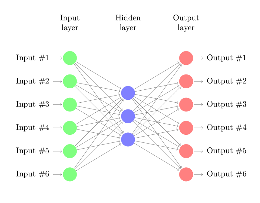
One can use an auto-encoder to detect outliers. An auto-encoder, also formerly called replicator network, is an unsupervised neural networks. Basically, it consists in learning a pair of non-linear transformations: A mapping from the original space to another space (encoder) - of possibly higher or lower dimensionality - and a mapping back from this new space to the original one (decoder). The assumption is, since outliers are rare and different, that the auto-encoder will not learn to map those objects correctly, inducing a higher reconstruction error. By looking at the reconstruction errors, one can infer an outlier score.

Interestingly, there is no need for labels, i.e. we don’t need to get example of normal and abnormal points. The network can infer directly from the data points a degree of abnormality with respect to the other points. This is what we may call a pure unsupervised setting. This is convenient in anomaly detection, because the characteristics of anomalies/outliers are in general not known in advance. It turns out that this method works quite well, as shown in previous work^{3 4 5}.

Nonetheless, high-dimensionality represents a major obstacle to outlier detection. Since auto-encoder learn a mapping to a possibly lower space, there are good reasons to think they would scale to high-dimensional problems. Unfortunately, such aspect was overlooked in the existing literature. Also, the typical benchmark data sets are low dimensional (with a maximum of 30 to 40 dimensions).

So, let’s try out. We are using one of the HiCS¹ synthetic data sets. The data set contains 100 dimensions and 1000 instances, with 136 of them being outliers. The data was generated such that outliers are hidden, i.e. they are visible only in particular subspaces. In the example above, we actually looked at the subspace [30,31,32] of this data set, which contains 5 outliers.

Let’s open the data set as a Pandas.DataFrame:

from scipy.io import arff
import pandas as pd 

data, meta = arff.loadarff("synth_multidim_100_000.arff")
data = pd.DataFrame(data)

We preprocess and save the labels for later. Note that we delete the labels from the original data set, because training with them would be like cheating !

labels = data['class'].astype(int)
labels[labels != 0] = 1
del data['class']

We normalize the data between 0 and 1:

from sklearn import preprocessing

min_max_scaler = preprocessing.MinMaxScaler()
np_scaled = min_max_scaler.fit_transform(data)
data_n = pd.DataFrame(np_scaled)
data_n = data_n.astype('float32')

Now we can start building a simple autoencoder. In this example, we will use Keras. We build an autoencoder with a single hidden layer containing 80 neurons, and an input and output layer of size 100. We use ReLU as activation function in the hidden layer and Sigmoid in the output layer. We choose adadelta as gradient optimizer and binary_crossentropy as loss function.

With just a few lines of code, we can starting training this network.

from keras.layers import Input, Dense
from keras.models import Model

encoding_dim = 80 
input = Input(shape=(100,))
encoded = Dense(encoding_dim, activation='relu')(input)
decoded = Dense(100, activation='sigmoid')(encoded)
autoencoder = Model(inputs=input, outputs=decoded)

encoder = Model(inputs=input, outputs=encoded)

encoded_input = Input(shape=(encoding_dim,))
decoder_layer = autoencoder.layers[-1]
decoder = Model(inputs=encoded_input, outputs=decoder_layer(encoded_input))

autoencoder.compile(optimizer='adadelta', loss='binary_crossentropy')

autoencoder.fit(data_n.values, data_n.values,
                nb_epoch=2500,
                batch_size=100,
                shuffle=True,
                verbose=0)

We train over 2500 epochs, with a batch size of 100. Finally, we get the prediction of the network for our data:

encoded = encoder.predict(data_n.values)
decoded = decoder.predict(encoded)

We compute the euclidean distance from each point to its reconstruction. We use it as an outlier score:

import numpy as np

dist = np.zeros(len(data_n.values))
for i, x in enumerate(data_n.values):
    dist[i] = np.linalg.norm(x-decoded[i])

Then, to assess the quality of our outlier detector, we plot the ROC curve:

from sklearn.metrics import roc_curve, auc
import matplotlib.pyplot as plt

fpr, tpr, thresholds = roc_curve(labels, dist)
roc_auc = auc(fpr, tpr)

plt.figure(figsize=(10,6))
plt.plot(fpr, tpr, color='red', label='AUC = %0.2f)' % roc_auc)
plt.xlim((0,1))
plt.ylim((0,1))
plt.plot([0, 1], [0, 1], color='navy', linestyle='--')
plt.xlabel('False Positive rate')
plt.ylabel('True Positive rate')
plt.title('ROC Autoencoder 100-80-100 ReLU/Sigmoid synth\_multidim\_100\_000')
plt.legend(loc="lower right")
plt.show()

An area under the curve (AUC) of 0.91 is actually very good. As a comparison, state-of-the-art methods, such as HiCS¹, only obtain an AUC of about 0.8 on this data set.

It is interesting to plot the outlier scores of each single data point:

data['labels'] = labels
data['dist'] = dist

plt.figure(figsize=(10,7))
plt.scatter(data.index, data['dist'], c=data['labels'], edgecolor='black', s=15)
plt.xlabel('Index')
plt.ylabel('Score')
plt.xlim((0,1000))
plt.title("Outlier Score")
plt.show()
plt.show()

Dark points are the outliers, inferred from the labels. As we can see, they get in general a higher score than non-outliers. The effect is even more visible if we compare the distance before and after learning. Before learning, the network weights are initialized randomly. The network has not learned any transformation yet so it performs very poorly at the reconstruction of each data points, independent of them being outliers or not.

Interpretability

The outlier score is a useful information about the abnormality of data points. However, in practice this is often not enough. One does not only want to know which points are outliers, but also why these points are so special, i.e. in which subspaces they are abnormal.

The lack of interpretation possibilities has been a major criticism of neural network. Neural networks are often seen as a magic black box doing great things but excluding any interpretation possibilities. I would say that in the case of outlier detection, this is not true.

By looking at the reconstruction error, we can find hints about the dimensions in which a particular data point is outlying. For example, point 350 is one of the outlier in the subspace [30,31,32], we can compute its reconstruction error per dimension and plot it:

def compute_error_per_dim(point):
    p = np.array(data_n.iloc[point,:]).reshape(1,100)
    encoded = encoder.predict(p)
    decoded = decoder.predict(encoded)
    return np.array(p - decoded)[0]

plt.figure(figsize=(12,7))
plt.plot(compute_error_per_dim(350))
plt.xlim((0,100))
plt.xlabel('Index')
plt.ylabel('Reconstruction error')
plt.title("Reconstruction error in each dimension of point 350")

As we can see, the point 350 shows a higher reconstruction error in dimensions [30,31,32], suggesting correctly that it is outlying in this subspace.

Similarly, point 50, which is an outlier in subspace [30,31,32] and [68,69], shows a high reconstruction error in dimensions [30,31,32,68,69].

Point 50 also has a relative high reconstruction error in subspace [50,51,52]. This is a false positive, because point 50 does not show a clear outlier behavior in this subspace. Still, it seems that point 50 is located in a relatively sparse region in the subspace [50,51,52] (see the red point).

So it seems that one can find back the information in which each object is an outlier by looking at the reconstruction errors, or at least reduce drastically the search space. Hereafter, we plot the reconstruction error of each outlier in the subspace [30,31,32]. Namely, the points 50, 121, 350, 572 and 559.

# 50, 121, 350, 572 and 559 are outliers in subspace [30,31,32]
plt.figure(figsize=(12,7))
plt.xlim((0,100))
plt.plot(range(100), compute_error_per_dim(50), label="50")
plt.plot(range(100), compute_error_per_dim(121), label="121")
plt.plot(range(100), compute_error_per_dim(350), label="350")
plt.plot(range(100), compute_error_per_dim(572), label="572")
plt.plot(range(100), compute_error_per_dim(669), label="669")
plt.legend(loc=1)
plt.xlabel('Index')
plt.ylabel('Reconstruction error')
plt.title("Reconstruction error in each dimension of outliers in [30,31,32]")

The peak at [30,31,32] seems quite consistent for each point.

What about Deep Learning?

Nowadays, everybody is crazy about deep learning. Increasing the size of a neural network is often thought as a silver bullet to increase accuracy. Despite being true in many settings, and especially in computer vision tasks, this is not true here.

For example, having to many parameters would allow the network to overfit the data, such that all points would be reconstructed nearly perfectly, blurring out the differences between normal and abnormal data points. Previous work⁴ showed that one single layer brings better results in outlier detection. Controversely, ⁵ argue that adding layers to compress gradually representation of the data helps. Obviously, there is a need for experiments here.

By chance, deep learning research leads the development of many gradient optimization and regularization methods that can be very useful for this task too.

Conclusion

In this article, we introduced the problems related to finding outlier in high-dimensional spaces. We show that neural-based approaches, such as auto-encoders, can provide great results.

Nonetheless, the quality of these results is conditioned by the choice of the parameters, such as the number of hidden neurons, activation function, gradient optimization, number of training epochs, size of mini-batches, distance function… Most of the current work is based on trial-and-error, which is time consuming and may lead to poor generalization. It would be interesting to derive rules to fix these parameters based on the data, such as its correlation structure or the expected proportion/characteristics of outliers.

The results showed in this article are based on a single data set, with carefully chosen parameters. It would be difficult to infer the quality of the same model on different data sets with different characteristics. Other neural-based methods, such as the Self-Organizing Maps⁶ or the Restricted Boltzmann Machines⁷ also shows promising results and would be interesting to compare.

Try it yourself !

The underlying notebook is available on my github, here. You are welcome to try out and play around with the parameters. Don’t hesitate to share your results if you find something interesting !

Sources