Data Stream Generation with Concept Drift

Concept drift is a well-known issue in the data stream community. It means that the statistical properties of a data stream can change over time in unforeseen ways. In this article, I will talk about concept drift and its relation to the outlier detection problem. I will also introduce a prototype in R that can be used to simulate several kinds of drift.

What is Concept Drift?

Concept drift has become a buzzword in data stream mining. It means that a change occurs in a time-dependent data flow, such that the description (either statistical or informal, qualitative) of concepts that are known currently might change in the future. This is interesting, because it can be understood intuitively. For example, in cyber-security the nature of cyber-attacks might change over time. It is a consequence of security patches, making selected attack vectors unusable, or new software introducing so far unknown security faults. As a result, the statistical properties of the underlying data change, and the anomaly detection models trained on aging data might show a loss in precision on new instances, if they are not correctly adapted.

Concept drift can be characterized differently, depending on its properties. If concept drift affects the boundaries of an underlying learning algorithms - i.e., the posterior probabilities have changed - it is said to be real. On the contrary, if it is not influencing the decision boundaries it is virtual.

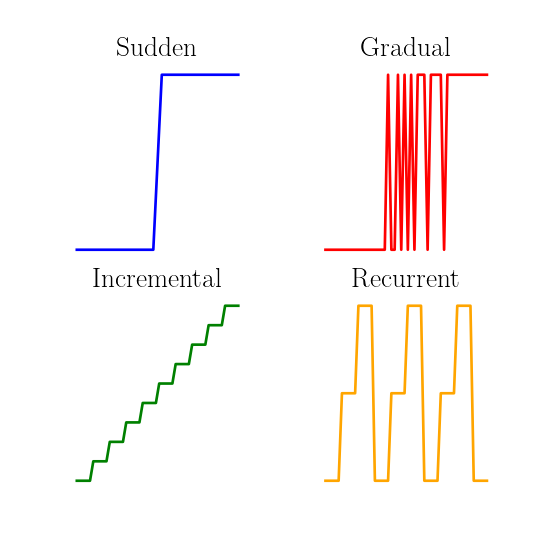
Concept drift can also be of different types:

• Sudden concept drift (sometimes called concept shift^{1 2}) characterizes abrupt changes of concepts.
• Gradual concept drift contains a transition phase, where the instances are generated by a mixture of a current concept and the next concept, and this proportion varies gradually through time until all instances are generated by the next concept.
• Incremental concept drift is characterized by a incremental modification of the current concept toward a future concept.
• Concept drift can be recurrent. It means that a concept from the past might reappear again in the future. This recurrence can be cyclic.
• Concept drift can be local or global³. Local concept drift affects only a small region of the feature space, and they are thus harder to detect than global drifts. Feature drift⁴ is also used to characterize drifts that affect only a subset of attributes.

The following figure illustrates the main types of concept drifts:

Quite often, concept drifts are a combination of all the above described types. Typically, concurrent drifts take place in multi-dimensional data streams and the characteristics of those drifts are unknown a priori.

From the literature, its seems that concept drift is quite well understood. This survey⁵ contains a rather compact description of the different types of concept drift, while this work⁶ provides a comprehensive taxonomy. In this survey⁷ also, the different approaches to adapt to concept drift are reviewed.

Concept Drift in Outlier Detection

Outlier detection can be considered as a subclass of the classification problem. Outlier detection is distinct from classification for the following reasons:

• The classes (outlier/non outlier) are highly imbalanced, since outliers are rare.
• There may not be a rule to describe all the outlying instances, because they can be outlying in different ways. Their common distinction is that they are different from other data points, in some way.
• The characteristics of outliers/anomalies are unknown beforehand. Which leads to the impossibility to rely completely on ground truth.
• In real-time setting, labels may not be available in a timely manner. One typically need to investigate first before declaring a point as an outlier.

As a result, outlier detection is often treated as an unsupervised problem.

Concept drift can impact outlier detection. For example, a point that may be considered as an outlier at time \(t_{1}\) may not be seen as an outlier at time \(t_{2}\) anymore.

There exist tools to generate data to reflect concept drift. The MOA⁸ framework includes several drifting data stream generators based for example on rotating hyperplanes or radial basis functions.

There exist also ways to generate data sets with outlier. The most common method is to start from a multi-class problem and to downsample one of the class. Then, the instances of this class become rare. Note that the relevance of such procedure in outlier detection is arguable, because all “outliers” are then tied to a same underlying concept: The class they originally belong to.

Nonetheless, there are - to the best of my knowledge - no generation procedure available to generate data with outliers subject concept drift. Particularly interesting are the so-called hidden outliers, because they can only be seen in particular subspace, so their detection is not trivial. I gave an example of what a hidden outlier is in a precedent article, that I am going to display here again:

In this 3-dimensional space, the points in red can be considered as hidden outliers, because they will be invisible as such in any 2-D or 1-D projections. Such outliers are in regions of relatively low density, but they cannot be detected in the full dimensional space because of the effects of the so-called curse of dimensionality, which destroys the notion of neighborhood⁹. To find them, one need to investigate particular subspaces. This is difficult, because the number of subspaces increases exponentially with the total number of dimensions.

In the following, we describe a data generator that simulates this kind of outliers, and where the dependencies in subspaces change such that the concept of outlier is drifting.

The Data Stream Generator

We create a number N of m-dimensional vectors. Their values are uniformly distributed between 0 and 1, except for selected subspaces, which show some kind of dependency, whose strength can change over time. To generate the dependencies, we take inspiration from the synthetic data used in the HiCS¹⁰ experiments, where dependencies are constructed by placing most data points close to the subspace axises, below a particular margin, creating an almost empty hypercube. Then, we let the size of this margin vary.

The following image illustrates a 2-D subspace where the strength of the dependency changes over time. Each image corresponds to a snapshot of the same stream at different time steps. As you can see, two outliers (in red) are visible in the third image.

Basically, points are generated independently, with respect to parameters that change over time, characterizing the current concept. The parameters consist mainly in a chosen set of subspaces \(S = {S_{1}, S_{2}, …, S_{i} }\) associated to a value between 0 and 1, the so-called margins \(M = M_{1}, M_{2}, …, M_{i}\). A smaller margin means a stronger dependency. For a number of iteration n, the procedure is the following:

• Generate a new m-dimensional vector whose values are taken uniformly from the range 0 to 1 for all m dimension.
• For each subspace \(S_{k}\), the vector has a probability \(prop\) to become an outlier in this subspace.
• If the vector is an outlier in subspace \(S_{k}\). We scale the value of such outlier in \(S_{k}\) to make sure that it is at a certain distance from the margin (10% of the side of the hypercube). This hinders the creation of false positives.
• If the vector is not an outlier in subspace \(S_{k}\), it is moved uniformly into the margins. By uniformly, we mean that it has an equal chance to be projected in any part of the denser area, to make sure that its density stays uniform.

For a number of step \(nstep\), the set \(S\) is modified randomly and the value in \(M\) incremented/decremented uniformly to reach after a number of iteration n the value fixed at the next step. The result is a data stream where hypercubes of variable size in selected subspaces are formed, which potentially contain outliers. Note that the probability to find outliers in the hypercubes is proportional to the volume of the hypercube.

The speed at which the parameters are changed is controlled by the number of point at each step \(N = {n_{1}, n_{2}, …, n_{nstep}}\) and the \(volatility\), i.e. the number of subspaces whose margin value change at each step. At the end of the generation, the labels for the produced outliers are available and contain the information in which subspace they are visible.

The generator is distributed on my GitHub as an R projet. It is powerful in a sense that it can generate high-dimensional data streams, where multiple local feature drifts occur at variable speed, from sudden to incremental. The concept drift can also be recurrent and the recurrence can be cyclic. This type of concept drift can be considered as real because the distribution of the outliers (that we try to predict) is changing with the drift. More information about the technical details of the project can be found in the GitHub page.

Future work

This work will be extended. It would be for example interesting to support different kind of dependencies. Especially, there are dependencies that are difficult to spot using traditional correlation measures such as Pearson and Spearman coefficients.

For example, the following code in R generates a donut:

generateDonut <- function(margin=0.3){
  t <- 2*pi*runif(1)
  u <- (runif(1) + runif(1))
  ifelse(u>1, r <- 2-u, r <- u)
  if(r < margin){r <- (r*(1-margin)/margin) + margin}
  c(r*cos(t), r*sin(t))
}

data <- data.frame(t(replicate(1000, generateDonut())))
plot(data)

Such a subspace obtains very low correlation estimates with traditional correlation measures (Pearson, Spearman, Kendall), in the order of \(10^{-2}\). Nonetheless, a dependence obviously exists and there is space - for example in the center and corners - to place hidden outliers.

Also, in the current implementation, concept drift takes place uniformly from a specific margin value to a new nominal margin value. Such uniformity might be unrealistic. Instead, the change could take the shape of a sigmoidal function², for example.

Another interesting question is, how can we keep track of dependency changes in an unknown stream efficiently? In predictive maintenance, one is interested in maintaining a set of most relevant subspaces through time, while this relevance is likely to change. This is still an open research question.

Sources